As I promised some time ago, I will discuss some of the new features in gnuplot 4.4. The first one that I would like to show is the concept of iteration in the plot command, and the concept of certain pseudo-files. If you have ever had to script the creation of your plots, you will appreciate these features.
First, let us see what the for loop looks like in the plot command. There are forms of it: once one can loop through integers, while in the other case, one can step through a string of words. So, the iteration either looks like
or
After this introduction, let us see how these can be used in real life. The first example that I will show is that of waterfall plots, i.e., when a couple of curves are plotted on the same graph, and they are shifted vertically. This is common practice, when one has several spectra, and wants to show the effect of some parameter on the spectra.
I would like to walk through the script line by line, for there is something unusual in almost each line. So, after re-setting the gnuplot session, we define a function, which will be a Gaussian, whose centre and width is determined by the parameter 'a'. We then plot this function to a file, 'iter.dat', and do it 6 times, and each time with a different parameter, so that the Gaussian is shifted, and becomes broadened. Note, however, that we do this by plotting a special file, '+'. This was introduced in gnuplot 4.4, and the purpose of this special file is that by invoking this, one can use the standard plot modifiers even with functions. I.e., we can specify 'using' for a function. The importance of this is that many plot styles require several columns, and we could not use those plot styles with functions without the '+' pseudo-file. Consider the following example
![]()
We can thus colour our curve by specifying the colour in the third column of the pseudo-file. Of course, this is only one possibility, and there are many more. If one wants to plot 3D graphs, then the pseudo-file becomes '++', but the concept is the same: the two variables are denoted by $1 and $2, and the function is calculated on the grid determined by the number of samples and the corresponding data range.
Now, back to the iteration loop! We produce 6 columns of data by plotting '+' by invoking a plot style that requires 6 columns. In this case, it is the xyerrorbars. Having created some data, we plot each column, but we call plot only once: the iteration loop does the rest. In each plot, the curve is shifted upwards, and the title is taken from the column number. For specifying the title, we use the function that we defined earlier: it takes an integer, and returns a string. At the end of the day, we have this graph
![]()
This was an example, when we plot various columns from the same file. We can also use the iteration to plot different files. When doing so, there are two options available. One is that we simply specify the file names in a string, as below
The second option is, if the data files are numbered, e.g., if we have 'file_1.dat', 'file_2.dat', and so on, we can use the iteration over integers as follows
First, let us see what the for loop looks like in the plot command. There are forms of it: once one can loop through integers, while in the other case, one can step through a string of words. So, the iteration either looks like
plot for [var = start : end {:increment}]
or
plot for [var in "some string of words"]
After this introduction, let us see how these can be used in real life. The first example that I will show is that of waterfall plots, i.e., when a couple of curves are plotted on the same graph, and they are shifted vertically. This is common practice, when one has several spectra, and wants to show the effect of some parameter on the spectra.
reset
f(x,a) = exp(-(x-a)*(x-a)/(1+a*0.5))+0.05*rand(0)
title(n) = sprintf("column %d", n)
set table 'iter.dat'
plot [0:20] '+' using (f($1,1)):(f($1,2)):(f($1,3)):(f($1,4)):(f($1,5)):(f($1,6)) w xyerror
unset table

set yrange [0:15]
plot for [i=1:6] 'iter.dat' u 0:(column(i)+2*i) w l lw 1.5 t title(i)
I would like to walk through the script line by line, for there is something unusual in almost each line. So, after re-setting the gnuplot session, we define a function, which will be a Gaussian, whose centre and width is determined by the parameter 'a'. We then plot this function to a file, 'iter.dat', and do it 6 times, and each time with a different parameter, so that the Gaussian is shifted, and becomes broadened. Note, however, that we do this by plotting a special file, '+'. This was introduced in gnuplot 4.4, and the purpose of this special file is that by invoking this, one can use the standard plot modifiers even with functions. I.e., we can specify 'using' for a function. The importance of this is that many plot styles require several columns, and we could not use those plot styles with functions without the '+' pseudo-file. Consider the following example
resetwhich produces the following graph
unset colorbox
unset key
set xrange [0:10]
set cbrange [0:1]
plot '+' using ($1):(sin($1)):(0.5*(1.0+sin($1))) with lines lw 3 lc palette, \
'+' using ($1):(sin($1)+2):($1/10.0) with lines lw 3 lc palette
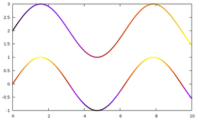
We can thus colour our curve by specifying the colour in the third column of the pseudo-file. Of course, this is only one possibility, and there are many more. If one wants to plot 3D graphs, then the pseudo-file becomes '++', but the concept is the same: the two variables are denoted by $1 and $2, and the function is calculated on the grid determined by the number of samples and the corresponding data range.
Now, back to the iteration loop! We produce 6 columns of data by plotting '+' by invoking a plot style that requires 6 columns. In this case, it is the xyerrorbars. Having created some data, we plot each column, but we call plot only once: the iteration loop does the rest. In each plot, the curve is shifted upwards, and the title is taken from the column number. For specifying the title, we use the function that we defined earlier: it takes an integer, and returns a string. At the end of the day, we have this graph

This was an example, when we plot various columns from the same file. We can also use the iteration to plot different files. When doing so, there are two options available. One is that we simply specify the file names in a string, as below
resetwhich will plot files 'first', 'second', 'third', 'fourth', and 'fifth'. At this point, note that 'file' is a string, i.e., we can manipulate it as a string. E.g., if we wanted to, instead of 'first', 'second', etc., plot 'first.dat', 'second.dat', and so on, we would do this as
filenames = "first second third fourth fifth"
plot for [file in filenames] file using 1:2 with lines
reset
filenames = "first second third fourth fifth"
plot for [file in filenames] file."dat" using 1:2 with lines
The second option is, if the data files are numbered, e.g., if we have 'file_1.dat', 'file_2.dat', and so on, we can use the iteration over integers as follows
resetwhich will plot the second column versus the first column of 'file_1.dat' through 'file_10.dat'.
filename(n) = sprintf("file_%d", n)
plot for [i=1:10] filename(i) using 1:2 with lines