Today I would like to touch on a vast subject, so prepare for a long post. However, I hope that the post will be worthwhile, for I want to discuss something that cannot be done in any other way. In due course, we will see how we can use gnuplot to create parametric plots from a file. What I mean by that is the following: if you want to plot, say, 10 similar objects, whose size is determined by the first column in a file. Of course, there are cases, when one can manipulate the size, e.g., if there is a pre-defined symbol, we can use one of the columns in a file to determine the size of the symbol. As an example, we can do this
So, let us get down to business! The first thing that I would like to discuss is the evaluate command. This is a really nifty way of shortening repetitive commands. Let us suppose that we want to place 10 arrows on our graph, and only the first coordinate of the arrows changes, otherwise everything is the same. Setting one arrow would read as follows
So, we have the evaluate command, and we have a new concept for functions. Then let us take a closer look at the following code
We will use this trick to create a parametric plot, taking parameter values from a file, first plotting the ellipses! Again, we have got to create some dummy data, and since we now need 6 columns, we will use the errorbars
First, we have the definition of a print function that looks rather ugly, but is quite simple. We want to plot
First we count, then plot g(x). At this point, we have the string that we need. We only have to set up our plot. Remember, we have a parametric plot, where the range of one of the variables is in [0:2*pi], while the other one is in [0:1]. Easy. Then we just have to evaluate our plot string, and we are done. Look what we have made here: a six-dimensional plot!
![]()
I think that this script is much less complicated, than many that we have discussed in the past. Short and clear, thanks to the eval command, and the new concept of functions. Besides, we pulled off a trick that was impossible by other means. I started out saying that we will create bars and pie. I believe, having seen the trick, it should be quite simple now, but in case you insist on seeing it, I will discuss it in my next post.
plot 'foo' u 1:2:3 with point pt 6 ps varwhich will draw circles whose radius is given by the third column in 'foo'. This is all well, but it works for a limited number of cases only, namely, when there is a symbol to start out with. But what happens, if we want to draw an object that is not a symbol, e.g., arcs of a circle, whose angle is given by one of the columns in a file, or cylinders, whose height is a variable, read from a file. As you can guess from these two suggestions, what we will do is to draw a pie, and a bar chart. I understand that we have done this a couple of times before, but this time, we will stay entirely in the realm of gnuplot, and the scripts are really short. We just have to figure out what to write in the scripts. But beyond this, I will also show how we can plot in 6 dimensions. We will plot ellipses on a plane (first 2 columns), whose two axes are given by the 3rd and 4th axis, the orientation by the 5th, and the colour by the 6th. If you are really pressed for it, you can add three more dimensions: if you draw ellipsoids in 3D, take all three axes from a file, and also the orientation, that would make 9 dimensions altogether. Quite a lot!
So, let us get down to business! The first thing that I would like to discuss is the evaluate command. This is a really nifty way of shortening repetitive commands. Let us suppose that we want to place 10 arrows on our graph, and only the first coordinate of the arrows changes, otherwise everything is the same. Setting one arrow would read as follows
set arrow from 0, 0 to 1, 1Of course, there are quite a few settings that we could specify, but this was supposed to be a minimal example. Then, the next arrow should be
set arrow from 1, 0 to 2, 1and so on. What if we do not want to write this line a thousand times, and we do not want to search for the coordinate that we are to change, the first one, in this case? We could try the following
a(x) = sprintf("set arrow from %d, 0 to %d, 1", x, x+1)
This function takes 'x', and returns a string with all the settings and coordinates. So, we are almost done. The only thing we should do is to make gnuplot understand that what we want it to treat a(x) as a command, not as a string. Enter the eval command: it takes whatever string is presented to it, and turns it into a command. Thus, the following script creates 5 arrows, all parallel to each other, and consecutively shifted to the rigtha(x) = sprintf("set arrow from %d, 0 to %d, 1", x, x+1)
eval a(0)
eval a(1)
eval a(2)
eval a(3)
eval a(4)
I believe, this is a much simpler and cleaner procedure, than thisset arrow from 0, 0 to 1, 1I should mention here that if chunks of a command are the same, another method of abbreviating them is to use macros. Those are disabled by default, so first we have to set it. Then it works as follows
set arrow from 1, 0 to 2, 1
set arrow from 2, 0 to 3, 1
set arrow from 3, 0 to 4, 1
set arrow from 4, 0 to 5, 1
set macroi.e., the term @ST is expanded using the definition above, therefore, this plot is equivalent to this one
ST = "using 1:2 with lines lt 3 lw 3"
plot 'foo' @ST, 'bar' @ST
plot 'foo' using 1:2 with lines lt 3 lw 3, 'bar' using 1:2 with lines lt 3 lw 3but the previous one is much more readable. I would also say that using capitals for the macros is probably not a bad idea, because then they cannot be mistaken for standard gnuplot commands. This much in the way of macros!
So, we have the evaluate command, and we have a new concept for functions. Then let us take a closer look at the following code
a(x) = sprintf("set arrow from %d, 0 to %d, 1;\n", x, x+1)
ARROW = ""
f(x) = (ARROW = ARROW.a(x), x)
plot 'foo' using 1:(f($1))
and let us suppose that our file 'foo' contains the following 5 lines1After plotting 'foo', the string 'ARROW' will be the following
3
5
7
9
set arrow from 1, 0 to 2, 1;I.e., we have a string, which contains instructions for setting 5 arrow. If, at this point, we simply evaluate this string, all 5 arrows will be set. Therefore, we have found a way of using a file to set the coordinates of an arrow. (N.B., if it was for the arrows only, we wouldn't have had to do anything, since there is a plotting style, 'with vector', as we discussed some weeks ago.)
set arrow from 3, 0 to 4, 1;
set arrow from 5, 0 to 6, 1;
set arrow from 7, 0 to 8, 1;
set arrow from 9, 0 to 10, 1;
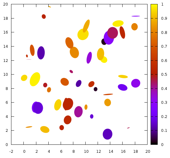
We will use this trick to create a parametric plot, taking parameter values from a file, first plotting the ellipses! Again, we have got to create some dummy data, and since we now need 6 columns, we will use the errorbars
resetwhich will produce 6 columns and 50 lines. Having produced some data, let us see what we can do with it. Here is our script:
f(x) = rand(0)
set sample 50
set table 'ellipse.dat'
plot [0:10] '+' using (20*f($1)):(20*f($1)):(f($1)):(f($1)):(3.14*f($1)):(f($1)) w xyerror
unset table
PRINT(x, y, a, b, alpha, colour) = \
sprintf("%f+v*(%f*cos(u)*cos(%f)-%f*sin(u)*sin(%f)),
%f+v*(%f*cos(u)*sin(%f)+%f*sin(u)*cos(%f)),
%f with pm3d", x, a, alpha, b, alpha, y, b, alpha, b, alpha, colour)
PLOT = "splot "
num = -1
count(x) = (num = num+1, 1)
g(x) = (PLOT = PLOT.PRINT($1, $2, $3, $4, $5, $6), \
($0 < num ? PLOT=PLOT.sprintf(",\n") : 1/0))
plot 'ellipse.dat' u 1:(count($1))
plot 'ellipse.dat' using 1:(g($1))

unset key
set parametric
set urange [0:2*pi]
set vrange [0:1]
set pm3d map
set size 0.5, 1
eval(PLOT)
First, we have the definition of a print function that looks rather ugly, but is quite simple. We want to plot
a*v*cos(u), b*v*sin(u), colourwhere a, and b are the axes of the ellipse, and colour is going to specify, well, its colour. However, we want to translate the ellipse to its proper position, and we also want to rotate it by an amount given by the 5th column, so we have to apply a two-dimensional rotation on the object. Therefore, we would end up with a function similar to this
x+v*(a*cos(u)*cos(alpha)-b*sin(u)*sin(alpha)), y + v*(a*cos(u)*sin(alpha)+b*sin(u)*cos(alpha)), colourNow you know why that print function looked so complicated! After this, we define a string, PLOT, that we will expand as we read the file. But before that, we have to count the lines in the file. The reason for that is that successive plots must be separated by a comma, but there shouldn't be a comma after the last plot. So, we just have to know where to stop placing commas in our string. Then we define the function that does nothing useful, but concatenates the PLOT string as it reads the file. Here we use the number of lines that we determine in a dummy plot. At this point we are done with the functions, all we have to do is plotting.
First we count, then plot g(x). At this point, we have the string that we need. We only have to set up our plot. Remember, we have a parametric plot, where the range of one of the variables is in [0:2*pi], while the other one is in [0:1]. Easy. Then we just have to evaluate our plot string, and we are done. Look what we have made here: a six-dimensional plot!
I think that this script is much less complicated, than many that we have discussed in the past. Short and clear, thanks to the eval command, and the new concept of functions. Besides, we pulled off a trick that was impossible by other means. I started out saying that we will create bars and pie. I believe, having seen the trick, it should be quite simple now, but in case you insist on seeing it, I will discuss it in my next post.