Chris asked an interesting question today, namely, how one can restrict the fit range in gnuplot. What he meant by that was not the range of the data points (that is really easy, the syntax is the same as for plot), but the range of fit parameters. In some cases, it is a quite reasonable requirement, because we might know from somewhere that certain parameter values just do not make any sense. As it turns out, it is rather easy to achieve this in gnuplot. All we have to do is to come up with a function that restricts its values in the desired range.
After this interlude, let us see an example! We will create some data with the following gnuplot script:
We take a Gaussian, with some noise added to it. Naturally, we would like to fit a Gaussian to this data, and in particular, f(x). But what, if our model is such that 'a' must be in the range [1.1:2], 'b' must be in the range [0.1:0.9], and 'c' must be in the range [0.5:1.5]? We just use in our fit, instead of f(x), another function, g(x), say, of the form
![]()
The point here is that as x runs from negative infinity to positive infinity, A(x) runs between 1.1, and 2.0, and likewise for B(x), and C(x). Then the fit goes on as it would normally. Our script is, thus, the following in its full glory:
and it produces the following graph:
![]()
At this point, we should not forget, that what we are interested in is not the value of 'aa', 'bb', or 'cc', but the value of 'a', 'b', and 'c'. This means that what we have to take is
A(aa), B(bb), and C(cc). If you print the values of 'a', 'b', and 'c' from the fit to f(x), the value of 'aa', 'bb', and 'cc', and the value of A(aa), B(bb), and C(cc), we get the following results
Obviously, the second print does not make too much sense, we have to compare the last one to the first one. We can here see that we got values in the ranges [1.1:2], [0.1:0.9], and [0.5:1.5], as we wanted to.
After this interlude, let us see an example! We will create some data with the following gnuplot script:
reset
a=1.0; b=1.0; c=1.0
f(x) = a*exp(-(x-b)*(x-b)/c/c)
set table 'restrict.dat'
plot [-2:4] f(x)+0.1*(rand(0)-0.5)
unset table
We take a Gaussian, with some noise added to it. Naturally, we would like to fit a Gaussian to this data, and in particular, f(x). But what, if our model is such that 'a' must be in the range [1.1:2], 'b' must be in the range [0.1:0.9], and 'c' must be in the range [0.5:1.5]? We just use in our fit, instead of f(x), another function, g(x), say, of the form
g(x) = A(a)*exp(-(x-B(b))*(x-B(b))/C(c)/C(c))where A(a), B(b), and C(c) take care of our restrictions. These functions are somewhat arbitrary, but for better or worse, I will take the following three arcus tangents
# Restrict a to the range of [1.1:2]which would look like this
A(x) = (2-1.1)/pi*(atan(x)+pi/2)+1.1
# Restrict b to the range of [0.1:0.9]
B(x) = (0.9-0.1)/pi*(atan(x)+pi/2)+0.1
# Restrict c to the range of [0.5:1.5]
C(x) = (1.5-0.5)/pi*(atan(x)+pi/2)+0.5

The point here is that as x runs from negative infinity to positive infinity, A(x) runs between 1.1, and 2.0, and likewise for B(x), and C(x). Then the fit goes on as it would normally. Our script is, thus, the following in its full glory:
# Restrict a to the range of [1.1:2]
A(x) = (2-1.1)/pi*(atan(x)+pi/2)+1.1

# Restrict b to the range of [0.1:0.9]
B(x) = (0.9-0.1)/pi*(atan(x)+pi/2)+0.1

# Restrict c to the range of [0.5:1.5]
C(x) = (1.5-0.5)/pi*(atan(x)+pi/2)+0.5
a=0.0
b=0.5
c=0.9
fit f(x) 'restrict.dat' via a, b, c
g(x) = A(aa)*exp(-(x-B(bb))*(x-B(bb))/C(cc)/C(cc))
aa=1.5
bb=0.5
cc=0.9
fit g(x) 'restrict.dat' via aa, bb, cc
plot f(x), g(x), 'restrict.dat' w p pt 6
and it produces the following graph:
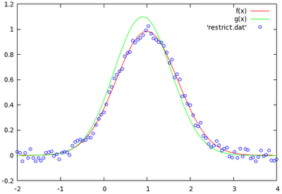
At this point, we should not forget, that what we are interested in is not the value of 'aa', 'bb', or 'cc', but the value of 'a', 'b', and 'c'. This means that what we have to take is
A(aa), B(bb), and C(cc). If you print the values of 'a', 'b', and 'c' from the fit to f(x), the value of 'aa', 'bb', and 'cc', and the value of A(aa), B(bb), and C(cc), we get the following results
gnuplot> pr a, b, c
0.984221984191135 0.996600824504231 1.00765240463672

gnuplot> pr aa, bb, cc
-3442408.91578921 1443864.45093385 -0.201236322474146

gnuplot> pr A(aa), B(bb), C(cc)
1.10000008322047 0.899999823634477 0.936788734177637
Obviously, the second print does not make too much sense, we have to compare the last one to the first one. We can here see that we got values in the ranges [1.1:2], [0.1:0.9], and [0.5:1.5], as we wanted to.